One of the simplest ecological population models is the exponential growth model \[N_{t+1} = \alpha \cdot N_t\] which indicates the rate of exponential increase (if \(\alpha > 1\)) or decrease (if \(0 \leq \alpha < 1\)) or stasis (if \(\alpha = 1\)).

Before going any futher lets put some R code in place to facilitate our exploration.

library(ggplot2)

update <- function(rule, ..., initial = 100, t = 100, rule_name = substitute(rule)) {
  for(i in 2:t) initial[i] <- rule(initial[i-1], ...)
  data.frame(t = 1:t, N = initial, rule = deparse(rule_name), ..., 
             initial = initial[1], stringsAsFactors = TRUE)
}

gp <- ggplot(mapping = aes(x = t, y = N)) +
  geom_line() +
  expand_limits(y = 0)

Now let us consider the population abundance over 100 time intervals from an initial value of 100 with \(\alpha\) values of 1.01, 1.00 and 0.99

exp_growth <- function(N, a) N * a

data <- rbind(update(rule = exp_growth, a = 1.01),
              update(rule = exp_growth, a = 1.00),
              update(rule = exp_growth, a = 0.99))

gp %+% data + facet_wrap(~a)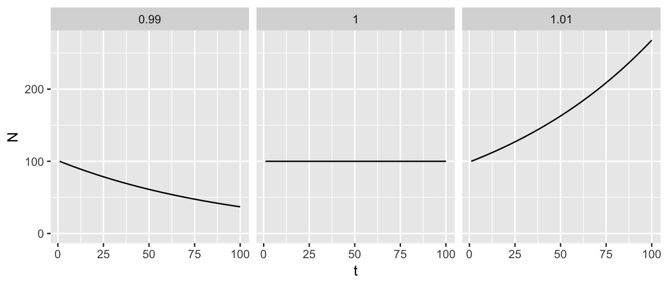

Although populations can in the short-term increase or decrease exponentially, density-dependence tends to limit the rate of change. The logistic difference equation adds a density-dependent term \(\beta\).

\[N_{t+1} = \alpha \cdot N_t - \beta \cdot N_t^2\]

One of the interesting things about the logistic difference model is the range of behaviours it displays (May 1976). Let us simplify our exploration by fixing \(\beta = 0.001\) and see how the population responds with different values of \(\alpha\).

log_diff <- function(N, a, b = 0.001) N * a - N^2 * b

data <- rbind(update(rule = log_diff, a = 2),
              update(rule = log_diff, a = 3),
              update(rule = log_diff, a = 3.1),
              update(rule = log_diff, a = 3.5),
              update(rule = log_diff, a = 3.6),
              update(rule = log_diff, a = 4))

gp %+% data + facet_wrap(~a)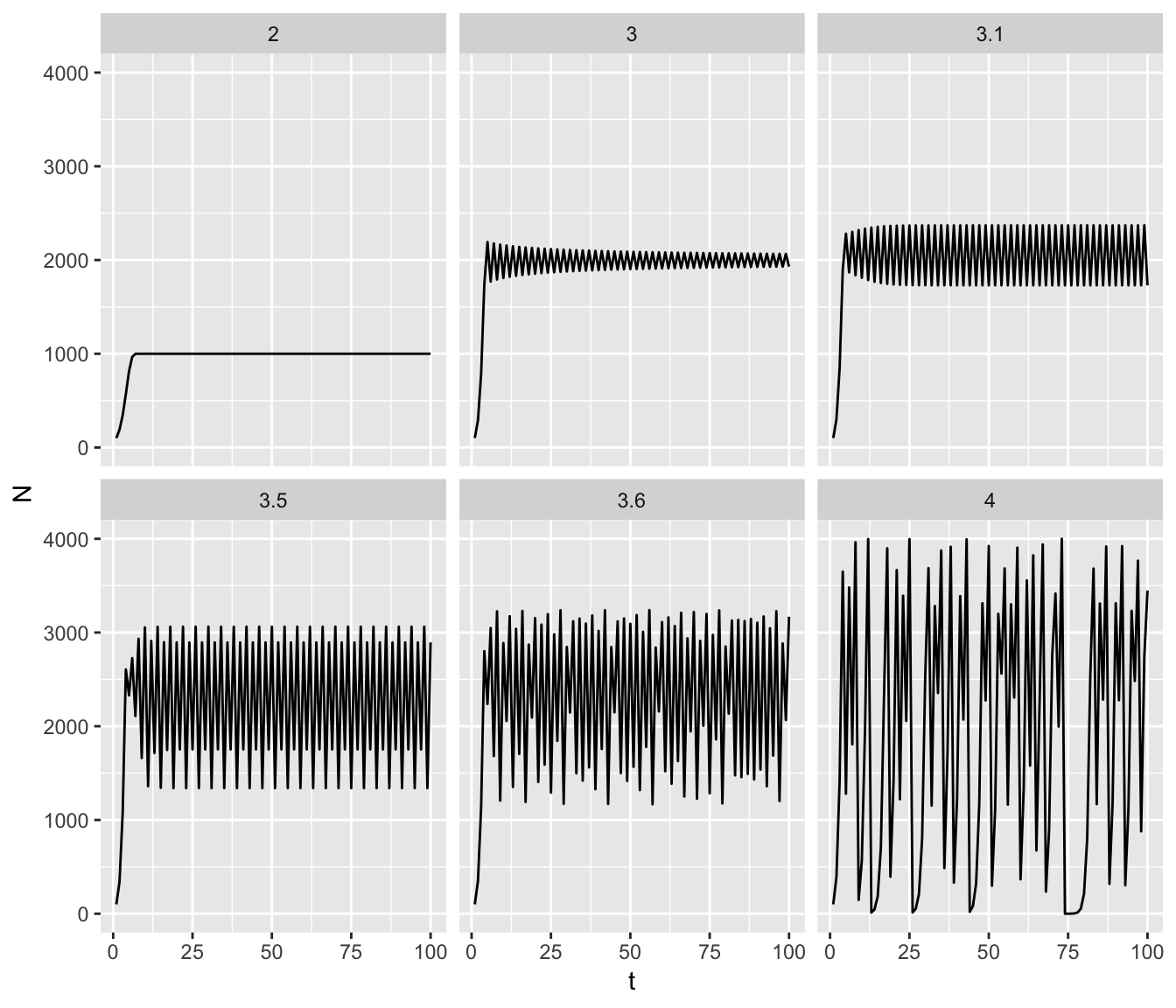

The results are fascinating. They range from monotonic damping, through damping oscillations, to stable limit cycles with increasing numbers of cycles before finally becoming chaotic (May 1976).

One of the most interesting things about chaos is that although it looks like stochastic noise the process that generates it is entirely deterministic¹.

Another interesting property of chaotic systems is their sensitivity to initial conditions(Lorenz 1963) aka the butterfly effect².

log_diff <- function(N, a, b = 0.001) N * a - N^2 * b

data <- rbind(update(rule = log_diff, initial = 100, t = 50, a = 4),
              update(rule = log_diff, initial = 100.0001, t = 50, a = 4))

data$initial <- factor(data$initial)

ggplot(data, mapping = aes(x = t, y = N)) +
  geom_line(aes(group = initial, color = initial)) +
  scale_colour_brewer(palette = "Set1")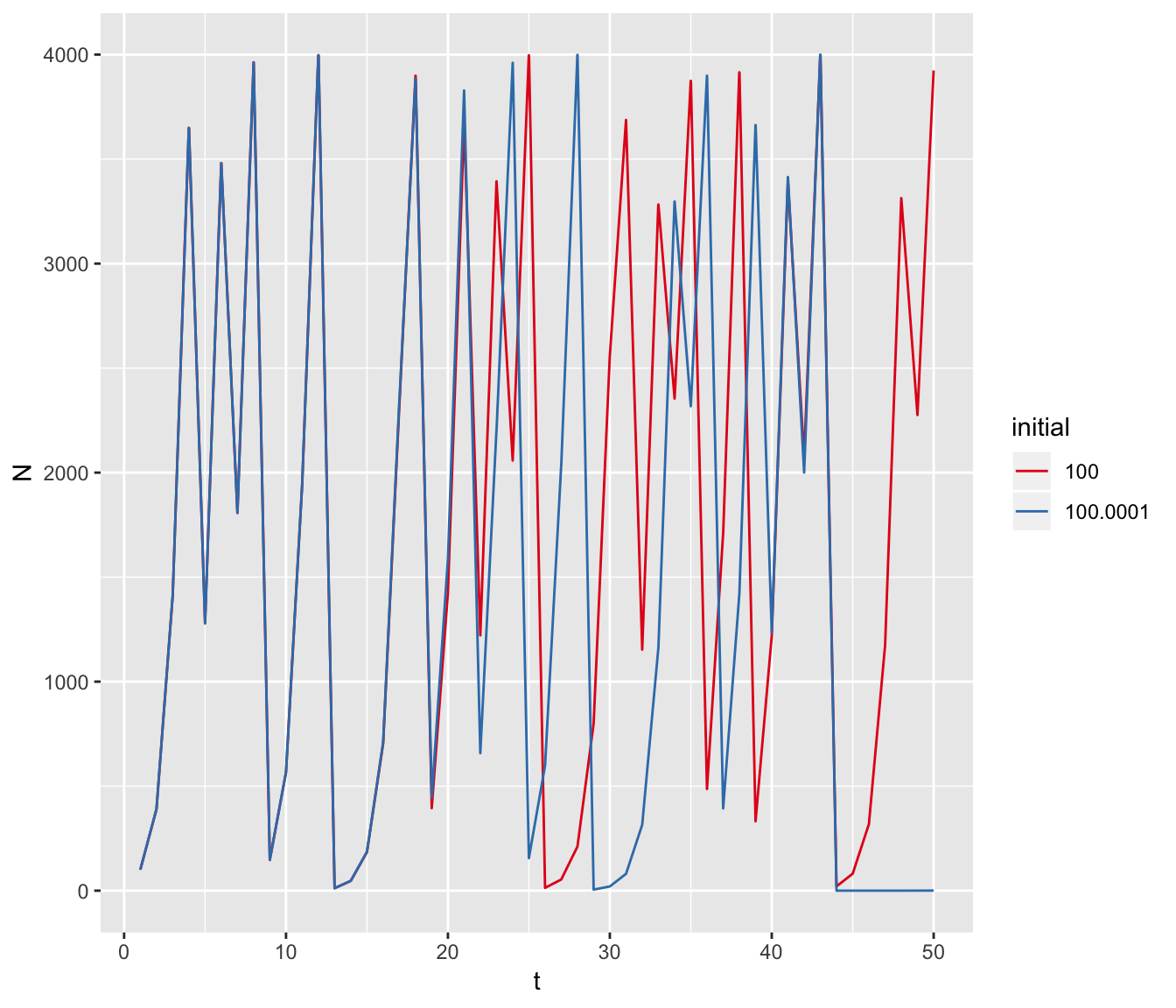

Consequences of this sensitivity include dramatically different outcomes from seemingly negligible changes as well as the impossibility of long-term predictions due to measurement error even when a system is fully understood!

References

Lorenz, Edward N. 1963. “Deterministic Nonperiodic Flow.” Journal of the Atmospheric Sciences 20 (2): 130–41. https://doi.org/10.1175/1520-0469(1963)020<0130:DNF>2.0.CO;2.
May, Robert M. 1976. “Simple Mathematical Models with Very Complicated Dynamics.” Nature 261 (5560): 459–67. https://doi.org/10.1038/261459a0.