Linear regression is of course defined by the certain relationship

\[\mu = \alpha + \beta \cdot x\] and the uncertain relationship

\[y \sim~ N(\mu, \sigma)\] where \(\alpha\) is the intercept and \(\beta\) is the slope.

For example with \(\alpha = 0\) and \(\beta = 10\) the deterministic relationship can be represented as follows

beta <- 10
x <- 0:10
mu <- beta * x
plot(x, mu, type = "l")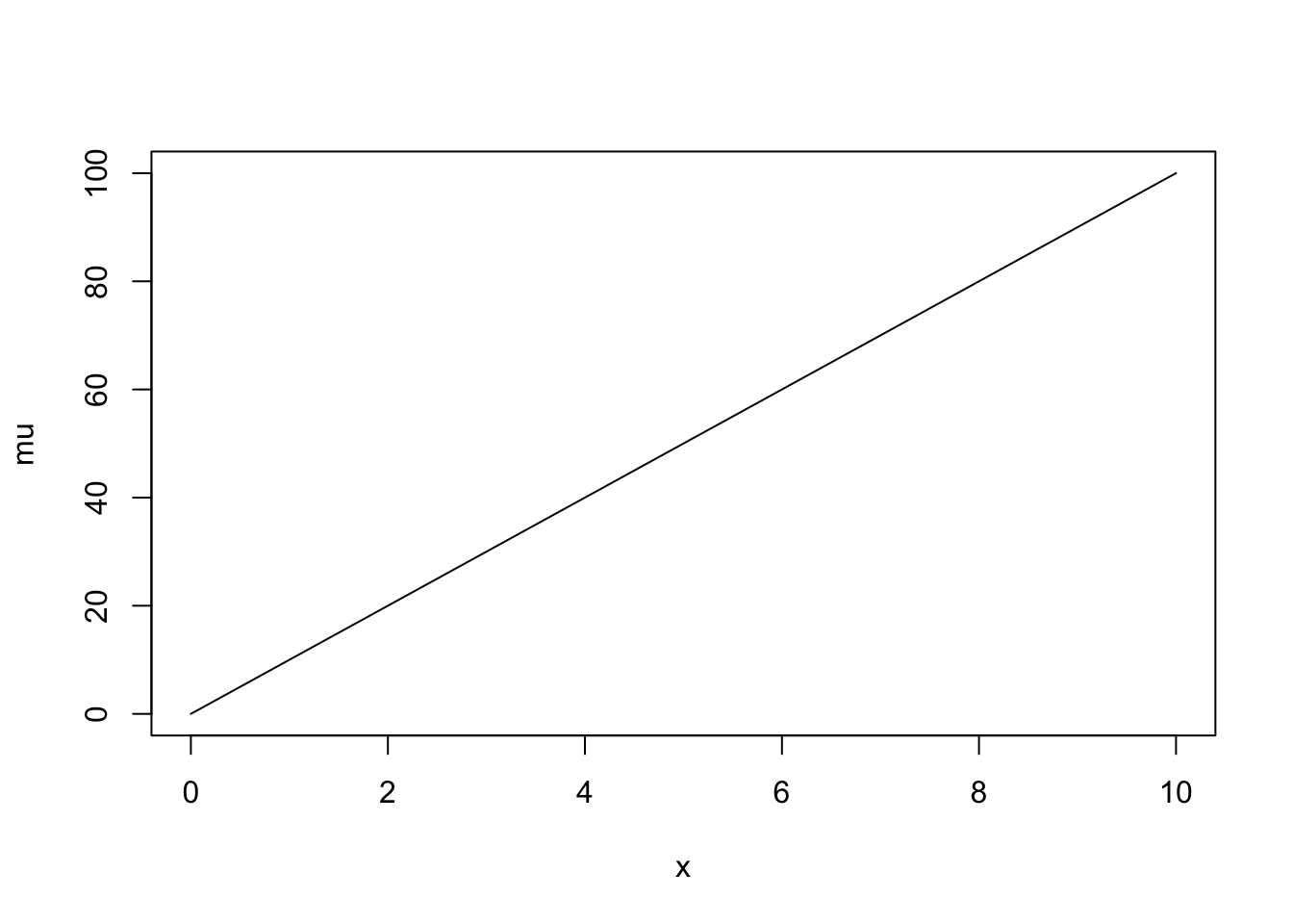

I was just thinking about how I would like the slope, ie \(\beta\), to vary with \(x\) and came up with the following certain relationship \[\mu = \alpha + (\beta + \beta_2 \cdot x) \cdot x\] which with \(\beta_2 = -0.5\) gives

beta2 <- -0.5
mu <- (beta + beta2 * x) * x
plot(x, mu, type = "l")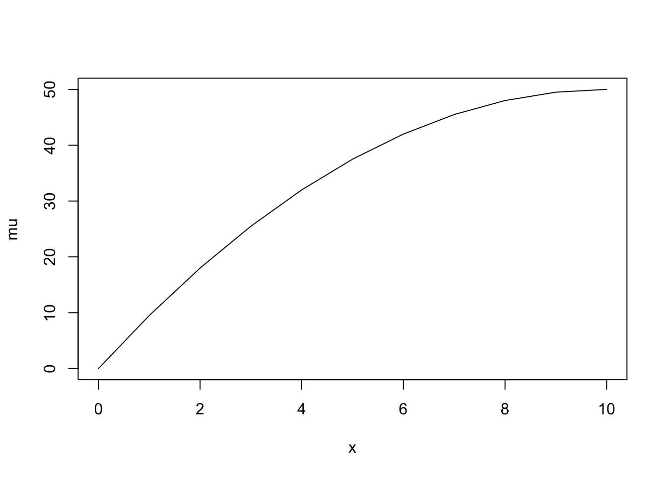

As I was admiring it I suddenly realized that it can be very simply rearranged to give \[\mu = \alpha + \beta \cdot x + \beta_2 \cdot x^2\] which is of course the standard polynomial relationship!

While this will be blindingly obvious to many it has somehow managed to elude me for many years. I’m not sure if I should feel exhilarated for having seen it or humiliated for having taken so long…