Often the concentration of a water quality parameter below a detection limit (DL) cannot be measured reliably.
A common approach to dealing with such non-detects is to substitute them with the value 0, DL/2 or DL which discards information and introduces biases.
A more reliable approach is to explicitly model the non-detects using censored probability distributions.
Simulated Data
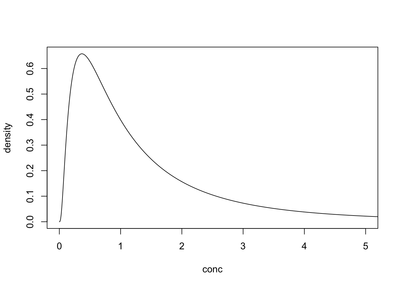
Consider the following log-normally distributed parameter (log mean of 0 and log SD of 1).
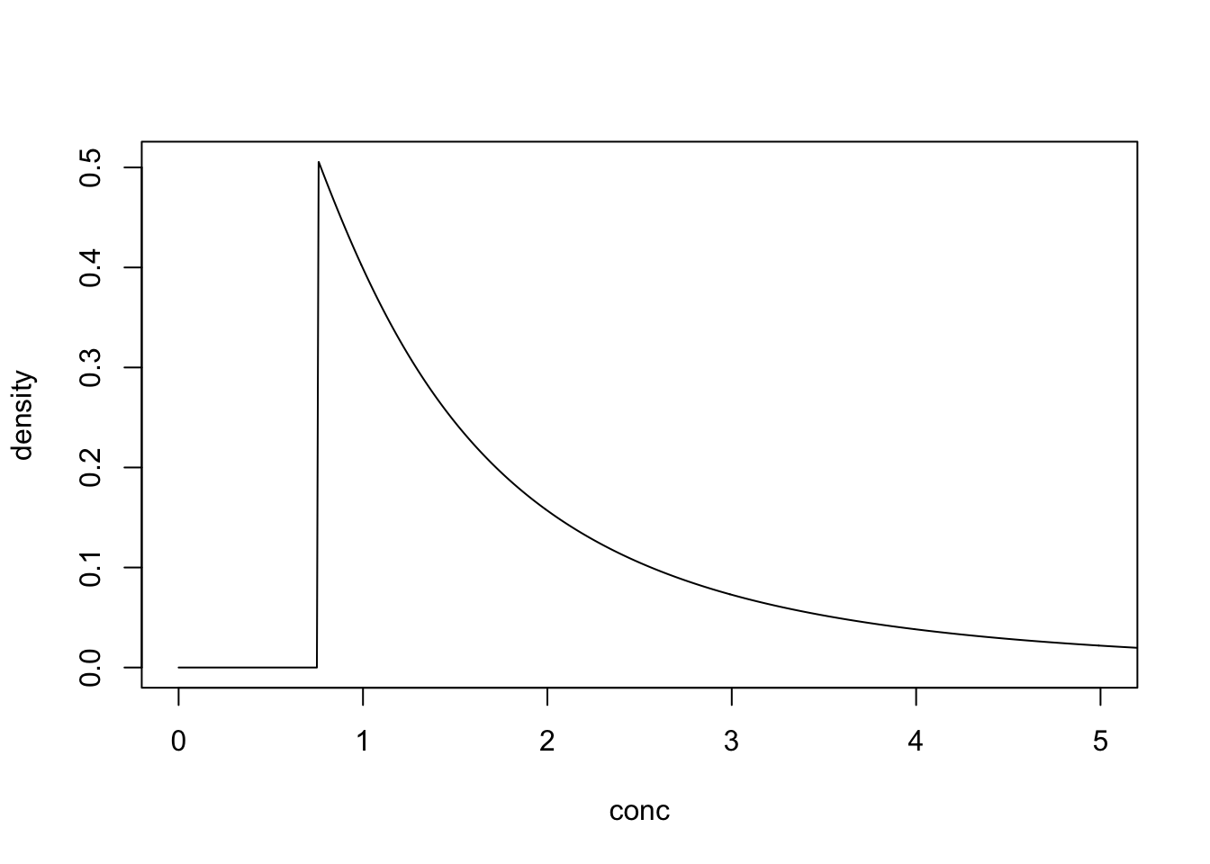
With a DL of 0.75 the detects would be distributed as follows.
Bayesian Analysis
Now let us analyse 1,000 simulated data points using the following Bayesian model.
model <- "model{
  log_mn ~ dnorm(0, 1)
  log_sd ~ dnorm(0, 1) T(0,)
  for(i in 1:length(Conc)) {
    Conc[i] ~ dlnorm(log_mn, log_sd^-2)
  }
}"
Reliable Detection
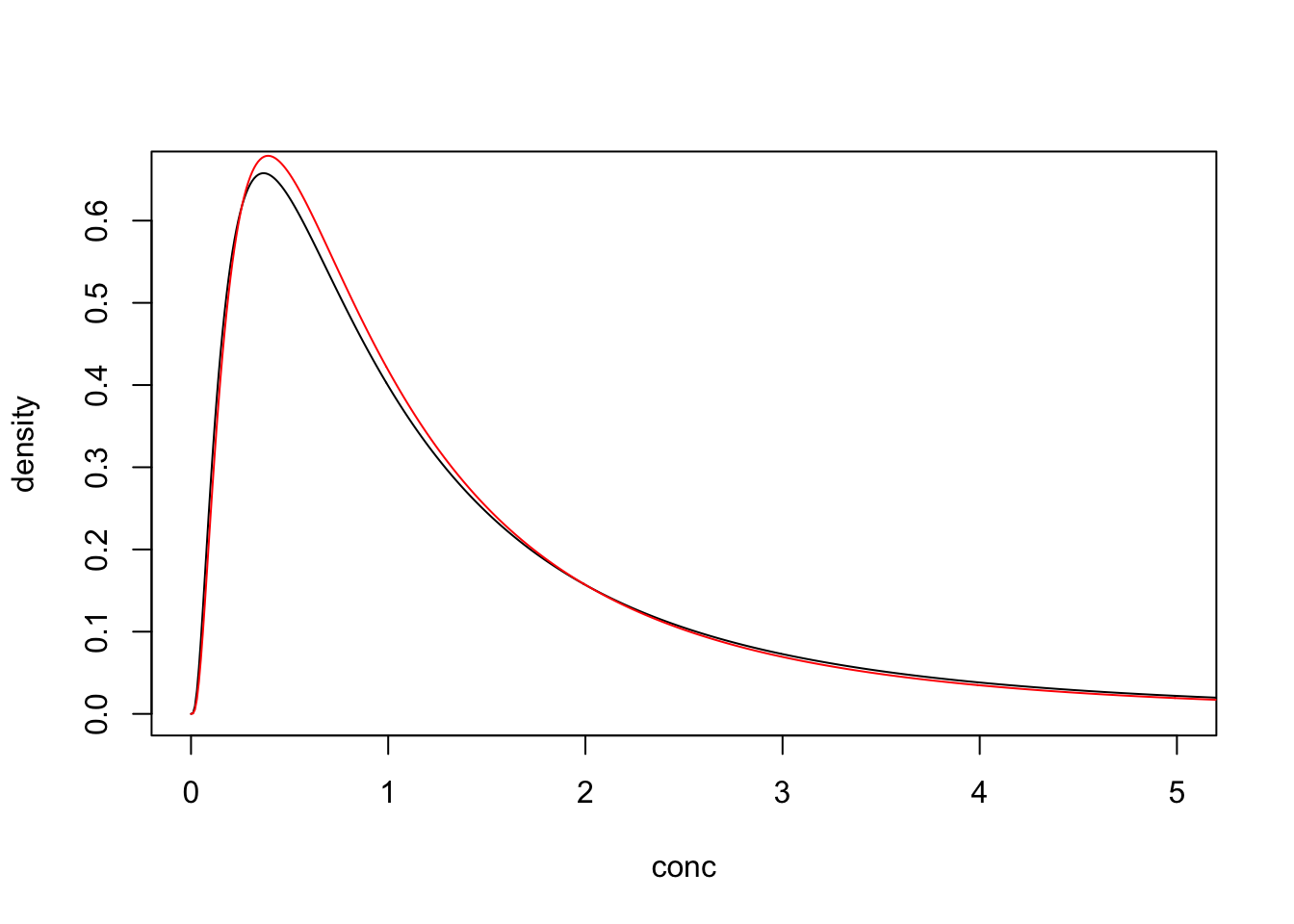
If there was no detection limit then any differences between the estimated (red) and underlying distributions (black) are due to sampling error.
##      log_mn      log_sd
## -0.03827642  0.96038244
Substitution
If, however, we had a detection limit of 0.75 and we substituted the non-detects for the DL then we would introduce an upwards bias.
##    log_mn    log_sd
## 0.2351745 0.6460452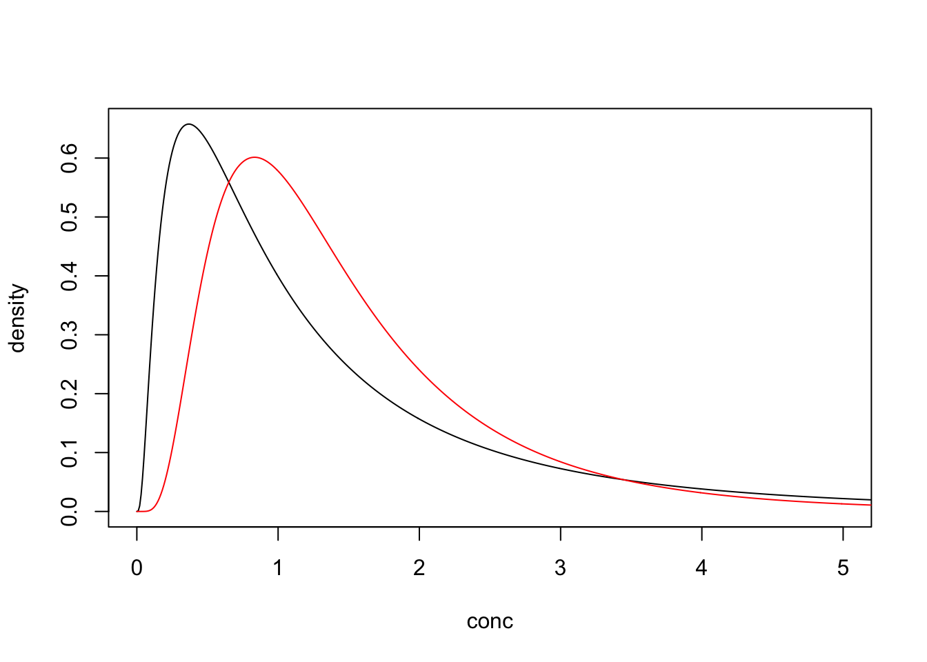
Missing Values
If we replaced the non-detects with missing values the bias would be even worse.
##    log_mn    log_sd
## 0.5697294 0.6322951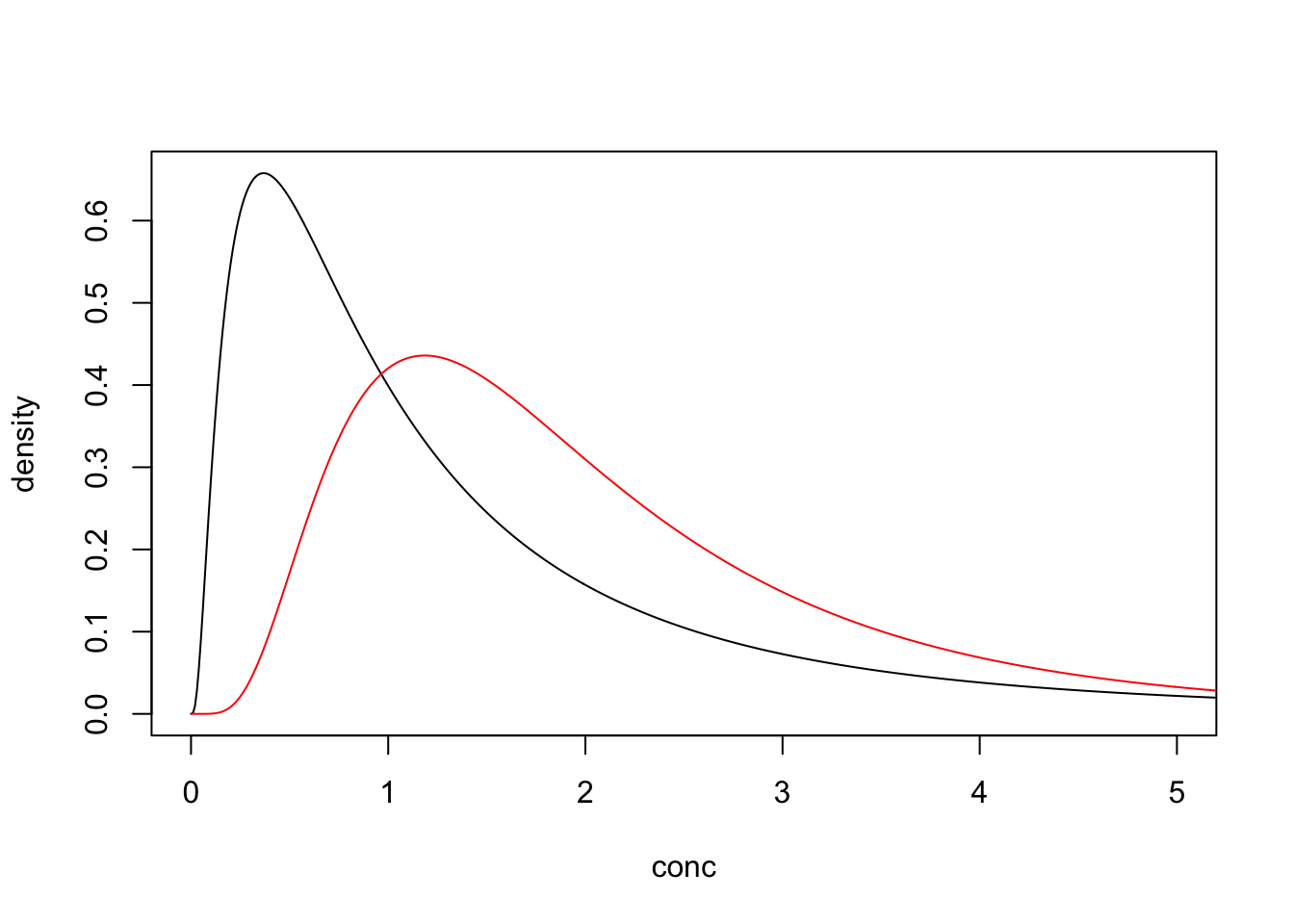
Censored Distribution
But if we also updated the model to include the interval() distribution and a indicator variable specifying which of the missing values are non-detects then the bias vanishes.
model <- "model{
  log_mn ~ dnorm(0, 1)
  log_sd ~ dnorm(0, 1) T(0,)
  for(i in 1:length(Conc)) {
    Conc[i] ~ dlnorm(log_mn, log_sd^-2)
    Indicator[i] ~ dinterval(Conc[i], c(0,0.75))
  }
}"
## log_mn log_sd
## -0.03030919 0.95506565
In the current example, the DL is a constant 0.75 but if it varied it would be necessary to pass the value for each observation in a third column.
Bayesian models provide a natural framework for modeling censored data because they readily handle missing values, easily incorporate multiple distributions and describe all the uncertainty.
Maximum-Likelihood Analysis
However, Bayesian models can be slow to fit and require the specification of prior distributions. Consequently, some users prefer maximum-likelihood (ML) models.
Censored Distribution
The final censored distribution can be refitted as an ML model using the NADA package in R.
library(NADA, warn.conflicts = FALSE)## Loading required package: survivaldata$Conc[is.na(data$Conc)] <- 0.75
mle <- with(data, cenmle(Conc, Indicator))## log_mn log_sd
## -0.02945614 0.95384629