The following was presented at the Columbia Mountains Institute’s conference on Regulated Rivers: Environment, Ecology, and Management in Castlegar, BC, which ran from May 6th to 7th, 2015. It is also provided below with additional text.
An Overview of the Statistical Challenges to Understanding the Ecology and Management of Regulated Rivers (with additional text)
Introduction
The statistical challenges associated with understanding the environment, ecology and management of regulated rivers are numerous. The challenges can be divided into data and analytic challenges. This document briefly defines and illustrates each of the challenges and provides recommendations for overcoming them. The challenges are illustrated using examples involving fish and discharge.
Data Challenges
There are at least seven types of data challenge:
- insufficient data
- missing data
- biased data
- erroneous data
- messy data
- undocumented data
- lost data
To understand the data challenges consider the following example fish and discharge dataset (Table 1) and simple (overly so!) linear regression model (Figure 1).
| Date | Discharge | Fish |
|---|---|---|
| 2010-01-01 | 1.10 | 0 |
| 2010-01-02 | 1.50 | 2 |
| 2010-01-03 | 3.00 | 5 |
| 2010-01-04 | 1.25 | 3 |
| 2010-01-05 | 1.05 | 1 |
| 2010-01-06 | 1.00 | 0 |
| 2010-01-07 | 1.30 | 0 |
| 2010-01-08 | 2.40 | 3 |
| 2010-01-09 | 1.20 | 1 |
| 2010-01-10 | 1.00 | 0 |
The linear regression yields the following significant (p = 0.001) result where the intercept is -1.74 and the slope 2.19 (Figure 1).
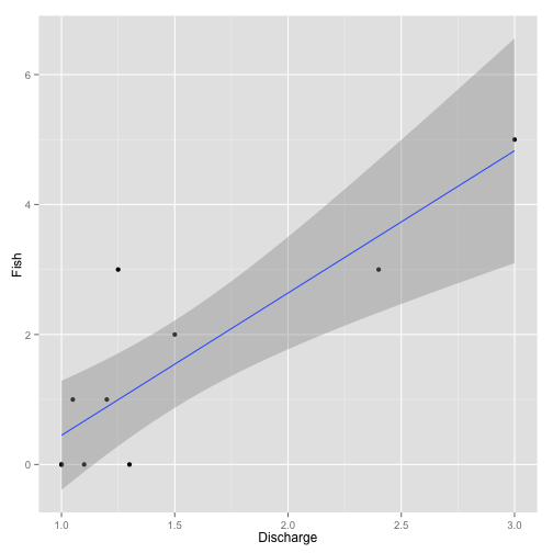
Figure 1. Example data analysis.
Insufficient Data
The challenge of insufficient data occurs when not enough data was collected to answer the question of interest (Table 2).
| Date | Discharge | Fish |
|---|---|---|
| 2010-01-01 | 1.1 | 0 |
| 2010-01-02 | 1.5 | 2 |
| 2010-01-03 | 3.0 | 5 |
In the example the result is no longer significant (p = 0.1; Figure 2). Reasons for insufficient data include a lack of appreciation of the variation in the data.
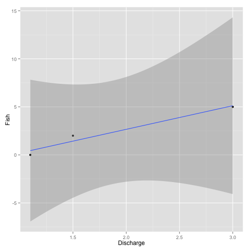
Figure 2. Example insufficient data analysis.
Missing Data
Although it can also result in a failure to answer the question of interest, missing data is different from insufficient data in the sense that it should have been collected but wasn’t (Table 3; Figure 3). The presence of missing data often requires special analytic techniques. Reasons for missing data include equipment failure and crew inattention.
| Date | Discharge | Fish |
|---|---|---|
| 2010-01-01 | 1.10 | 0 |
| 2010-01-02 | 1.50 | 2 |
| 2010-01-03 | NA | NA |
| 2010-01-04 | 1.25 | 3 |
| 2010-01-05 | 1.05 | 1 |
| 2010-01-06 | 1.00 | NA |
| 2010-01-07 | 1.30 | 0 |
| 2010-01-08 | 2.40 | 3 |
| 2010-01-09 | 1.20 | 1 |
| 2010-01-10 | NA | 0 |
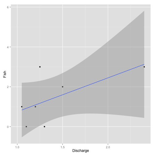
Figure 3. Example missing data analysis.
Biased Data
Although biased data also results from non-collection of data it is different from missing data in that the sense that the gaps are systematic (Table 4).
| Date | Discharge | Fish | |
|---|---|---|---|
| 2 | 2010-01-02 | 1.50 | 2 |
| 3 | 2010-01-03 | 3.00 | 5 |
| 4 | 2010-01-04 | 1.25 | 3 |
| 5 | 2010-01-05 | 1.05 | 1 |
| 8 | 2010-01-08 | 2.40 | 3 |
| 9 | 2010-01-09 | 1.20 | 1 |
As well as presenting the same challenges as missing data, biased data can also result in incorrect estimates even though the data points are themselves correct. Thus the regression model now estimates the slope to be 1.68 (Figure 4).
Biased data can result from non-random subsampling decisions.
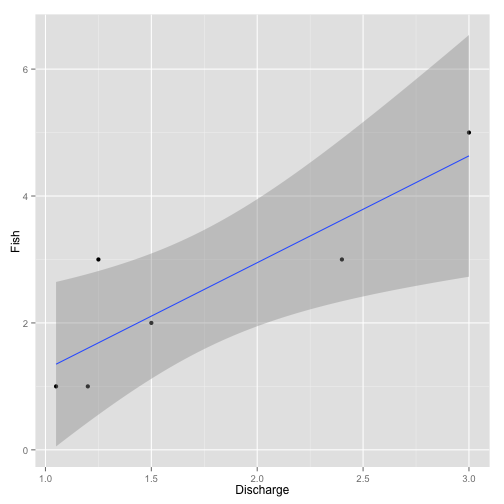
Figure 4. Example biased data analysis.
Erroneous Data
Like biased data, erroneous data can result in incorrect estimates although the problem is due to invalid data points as opposed to systematic gaps (Table 5). Equipment malfunction and crew inexperience are common causes of erroneous data. In the current example the slope is now estimated to be -2.19 (Figure 5)!
| Date | Discharge | Fish |
|---|---|---|
| 2010-01-01 | -1.10 | 0 |
| 2010-01-02 | -1.50 | 2 |
| 2010-01-03 | -3.00 | 5 |
| 2010-01-04 | -1.25 | 3 |
| 2010-01-05 | -1.05 | 1 |
| 2010-01-06 | -1.00 | 0 |
| 2010-01-07 | -1.30 | 0 |
| 2010-01-08 | -2.40 | 3 |
| 2010-01-09 | -1.20 | 1 |
| 2010-01-10 | -1.00 | 0 |
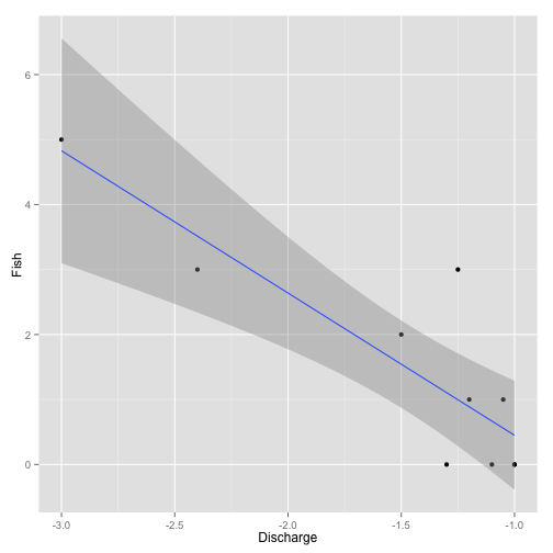
Figure 5. Example erroneous data analysis.
Messy Data
Wickham (2014) formally defined tidy data to be that for which:
- Each variable forms a column.
- Each observation forms a row.
- Each type of observational unit forms a table.
Messy data is by definition any other arrangement of the data (Table 6). Tidy data is easy to manipulate, model and visualize. Messy data must first be tidied.
| Day | 1 | 2 | 3 | 4 | 5 | 6 | 7 | 8 | 9 | 10 |
|---|---|---|---|---|---|---|---|---|---|---|
| Discharge | 1.1 | 1.5 | 3 | 1.25 | 1.05 | 1 | 1.3 | 2.4 | 1.2 | 1 |
| Fish | 0.0 | 2.0 | 5 | 3.00 | 1.00 | 0 | 0.0 | 3.0 | 1.0 | 0 |
Undocumented Data
Undocumented data is that for which no metadata exists (Table 7). The absence of metadata can prevent any sort of analysis or worse yet result in an inappropriate analysis being performed (Figure 6).
| Date | Q | F |
|---|---|---|
| 2010-01-01 | 1.10 | 0 |
| 2010-01-02 | 1.50 | 2 |
| 2010-01-03 | 3.00 | 5 |
| 2010-01-04 | 1.25 | 3 |
| 2010-01-05 | 1.05 | 1 |
| 2010-01-06 | 1.00 | 0 |
| 2010-01-07 | 1.30 | 0 |
| 2010-01-08 | 2.40 | 3 |
| 2010-01-09 | 1.20 | 1 |
| 2010-01-10 | 1.00 | 0 |
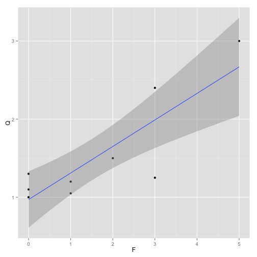
Figure 6. Example undocumented data analysis.
Lost Data
Lost data can be defined as data that was collected but no longer exists in paper or electronic form (Table 8).
| Date | Discharge | Fish |
|---|---|---|
| NA | NA | NA |
Data Solutions
Fortunately most of these data-related challenges can be overcome through recognition of the potential problems and a study design that includes where necessary a pilot study to identify all the data challenges; power analyses to ensure sufficient data are collected; equipment redundancy and specialized data collection and data entry forms so that the data are complete; field protocols that ensure unbiased subsampling; crew training and equipment redundancy so the data points are valid; a relational database so that the information is documented and tidy; and long-term data curation budgets so the information is archived for future use.
Analytic Challenges
There at least six types of analytic challenge
- vague questions
- hidden assumptions
- derived indices
- pseudo-replication
- over-reliance on significance testing
- researcher degrees of freedom
Vague Questions
An example of a vague question is
Does discharge affect fish abundance?
The question is obviously vague because it does not specify the species, life-stage or location (population). However nor does it specify the aspect of the hydrograph of interest (Olden and Poff 2003) identified 171 discharge metrics!) or the period of concern. It is also vague because it doesn’t specify how much of an effect is to be considered important.
Derived Indices
Derived indices are values which are calculated from other values without consideration of the underlying sampling distributions. For example the catch-per-unit-effort (CPUE) is
$$CPUE = \frac{Catch}{Effort}$$
However, analysing $CPUE$ (as opposed to $Catch$ and $Effort$) precludes
- use of a readily interpretable distribution, i.e.,
$Poisson$for$Catch$ - accounting for reduced uncertainty when lower effort
- testing for catch depletion
Pseudo-replication
Pseudo-replication occurs when replicates are not statistically independent, which is almost all the time in ecological studies! When determining the effect of discharge on fish abundance non-independence can occur due to repeated measures, individual longevity, recruitment, aggregations, invasive species, downstream effects and climatic effects on fish abundance and discharge.
Over-Reliance on Significance Testing
Often an effect is judged solely on its significance. However significance alone is a poor criterion because significant and insignificant effects can be large or small (Figure 7). A large insignificant effect is potentially much more important than a small significant one.
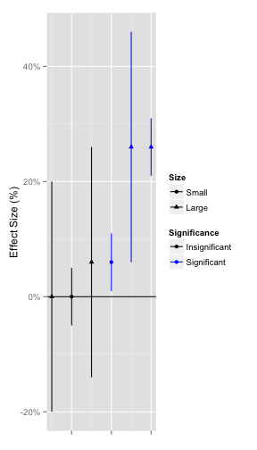
Figure 7. Various effect sizes.
Researcher Degrees of Freedom
Researcher degrees of freedom is an umbrella term for
all the data-processing and analytical choices researchers make after seeing the data.
A classic example is when researchers are tasked with identifying the environmental predictor variable(s) responsible for changes in the response. In the case of discharge and fish abundance the number of predictors can stretch into the tens or even hundreds. If 20 time series are considered the expectation is that one will predict the response by chance.
If researchers decisions are undocumented then the extent to which the probability of getting a false positive has been inflated cannot be assessed.
Analytic Solutions
Most of the analysis-related challenges can be overcome through hierarchical (account for non-independence), Bayesian scientific (explicitly describe observational and biological processes) models that allow the estimation of secondary parameters (answers to specific questions) with credible intervals (effect sizes) and the release of version-controlled code (researcher decisions).
References
Olden, Julian D., and N. L. Poff. 2003. “Redundancy and the Choice of Hydrologic Indices for Characterizing Streamflow Regimes.” River Research and Applications 19 (2): 101–21. https://doi.org/10.1002/rra.700.
Wickham, Hadley. 2014. “Tidy Data.” Journal of Statistical Software 59 (10): 1–22. http://www.jstatsoft.org/v59/i10.